Main menu
You are here
Linear Algebra in Engineering: Analyzing Dynamic Systems with Markov Chains (Part 6 of 7)
Preface
This series is aimed at providing tools for an electrical engineer to analyze data and solve problems in design. The focus is on applying linear algebra to systems of equations or large sets of matrix data.
Introduction
This article will demonstrate the use of Markov Chains. This can be used to analyze models with cyclic or or repeated outcomes.
If you are not familiar with linear algebra or need a brush up I recommend Linear Algebra and its Applications by Lay, Lay and McDonald. It provides an excellent review of theory and applications.
This also assumes you are familiar with Python or can stumble your way through it.
The data and code are available here: linear6.py and linear6.xlsx.
Concepts
Stochastic Model: a system or a model which includes random variables.
Stochastic matrix: describes a particular flow in statistical terms. For example they characterize the percentage of voters that switch or stick with their party (from year to year). Or the flow of people between cities. They are often annotated by the letter P. Stochastic matrices are probability matrices so columns must sum to exactly 1.
State Vector: describes the absolute state or value of a model. They are annotated with x.
Markov Chain: a stochastic model in which the probability of an event occurring is depends solely on the state attained in the previous event. A Markov chain is formed by calculating Px0. Subsequent calculations made by calculating Px0x1...xn.
Steady State Vector: a vector that is stable over time as n in xn approaches infinity. This is characterized by the equation Px=x.
Importing Your Data Set
I will use the Anaconda package suite with Python, numpy and the Spyder IDE for mathematical analysis. It is cross platform, free and open source. It is also easy to import data from Excel once you have the code snippet.
I usually have the following boilerplate code in my scripts:
import sys

import xlrd

import numpy as np

import matplotlib.pyplot as plt

from scipy.interpolate import interp1d
np.set_printoptions(threshold=np.nan)

print sys.version

print __name__
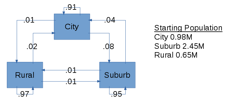
We read in two fixed sized arrays. One is a 3x3 stochastic model describing the flow of residents between City, Rural and Suburban areas of a metropolitan from one year to the next. The second describes a state vector of the population in each at the starting year.
filename='linear_6.xlsx'

print

print 'Opening',filename

ss=xlrd.open_workbook(filename,on_demand=True)

sheet_index=0

print ' Worksheet',ss.sheet_names()[sheet_index]

sh=ss.sheet_by_index(sheet_index)
print ' Reading data values'

stoch=[]

for row_index in range(0,sh.nrows):

    stoch.append([sh.cell_value(row_index,0),sh.cell_value(row_index,1),sh.cell_value(row_index,2)])

stoch=np.matrix(stoch)

print ' Stochastic model size:',len(stoch)

print

state0=[]

for row_index in range(0,sh.nrows):

    state0.append([sh.cell_value(row_index,4)])

state0=np.array(state0)

print ' State model size:',len(state0)
The last bit of code converts the array to a numpy matrix which will be necessary for the code below.
Numpy arrays are normally preferred but they do not support 'x*y' which will be handy here.
Calculating the Markov Chain
We need to calculate xi+1= Pxi.
print

print 'Stoch:'

print stoch

print 'State x0:'

print state0

print 'State x1:'

state1=stoch*state0

print state1

print 'State x2:'

state2=stoch*state1

print state2
This is the output:
2.7.11 |Anaconda 2.5.0 (64-bit)| (default, Jan 29 2016, 14:26:21) [MSC v.1500 64 bit (AMD64)]

__main__
Opening linear_6.xlsx

 Worksheet Sheet1

 Reading data values

 Stochastic model size: 3
State model size: 3
Stoch:

[[ 0.91  0.02  0.04]

 [ 0.01  0.97  0.01]

 [ 0.08  0.01  0.95]]

State x0:

[[  980000.]

 [ 2450000.]

 [  650000.]]

State x1:

[[  966800.]

 [ 2392800.]

 [  720400.]]

State x2:

[[  956460.]

 [ 2337888.]

 [  785652.]]
We can see the inflow/outflow of folks to City, Rural and Suburban areas from the starting year to the year after and the year after that.
Calculating the Steady State
If we continue calculating the Markov Chain over and over we will eventually reach steady state. I do this setting a maximum allowable error rate and calculating xi+1= Pxi over and over until the first entry in the state vector has an iteration to iteration error less than the maximum allowable.
The code for this is:
vector_sub1=[]

vector_sub2=[]

vector_sub3=[]

vector_error_sub1=[]

vector_error_sub2=[]

vector_error_sub3=[]

print

vector_sub1.append(state0[0])

vector_sub2.append(state0[1])

vector_sub3.append(state0[2])

vector_error_sub1.append([0])

vector_error_sub2.append([0])

vector_error_sub3.append([0])

max_error=1e-3

ss_state_prev=state0

ss_state_now=stoch*ss_state_prev

i=0

while abs(ss_state_prev[0]-ss_state_now[0]) > max_error:

    vector_sub1.append(ss_state_now[0])

    vector_sub2.append(ss_state_now[1])

    vector_sub3.append(ss_state_now[2])

    vector_error_sub1.append(ss_state_prev[0]-ss_state_now[0])

    vector_error_sub2.append(ss_state_prev[1]-ss_state_now[1])

    vector_error_sub3.append(ss_state_prev[2]-ss_state_now[2])

    i=i+1

    ss_state_prev=ss_state_now

    ss_state_now=stoch*ss_state_prev

print

print 'Max Error: ', max_error

print 'Final Error: ', ss_state_now[0]-ss_state_prev[0]

print 'Number of Iterations: ', i

print

print 'Steady State Vector:'

print ss_state_now
This code includes a bunch of extra arrays to plot error rates below.
The output:
Max Error:  0.001

Final Error:  [[ 0.00098843]]

Number of Iterations:  401
Steady State Vector:

[[ 1098461.5147391 ]

 [ 1020000.10675093]

 [ 1961538.37850993]]
Plotting code:
t=range(0,i+1)

plt.plot(t,vector_sub1,t,vector_sub2,t,vector_sub3)

plt.ylabel('# people')

plt.xlabel('time interval')

plt.show()

plt.clf()

plt.plot(t,vector_error_sub1,t,vector_error_sub2,t,vector_error_sub3)

plt.ylabel('error')

plt.xlabel('time interval')

plt.show()
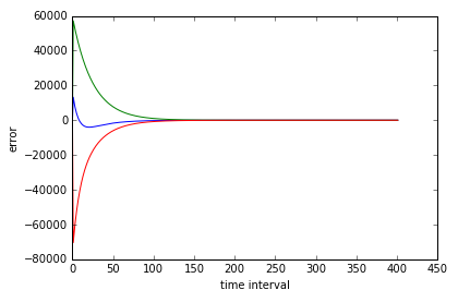
If we plot the state vectors and also the error these is what it looks like:
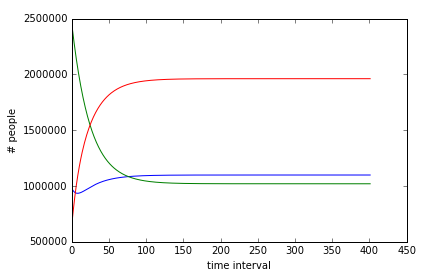
In the top graph you see all three variables asymptotically approach equilibrium as time approaches infinity.
In the bottom graph you can see the corresponding error approach zero as time approaches infinity.
Next Up
In the next article I will provide a summary of everything covered under Linear Algebra in Engineering.
- Log in to post comments