Linear Algebra in Engineering: Trend Analysis with Polynomial Least Squares (Part 2 of 7)

Preface
This series is aimed at providing tools for an electrical engineer to analyze data and solve problems in design. The focus is on applying linear algebra to systems of equations or large sets of matrix data.

Introduction
This article will demonstrate the use of least squares fit real data to a polynomial.

If you are not familiar with linear algebra or need a brush up I recommend Linear Algebra and its Applications by Lay, Lay and McDonald. It provides an excellent review of theory and applications.

This also assumes you are familiar with Python or can stumble your way through it.

The data and code are available here: linear2.py and linear2.xlsx.

Concepts
Interpolation: a method by which an equation is fitted to match a set of data. This equation relates the relationship of the variables in the data. This allows you to evaluate new data points not contained within a data set. It also allows you to evaluate and analyze the behavior of a system without actually measuring the system. Interpolated functions require an exact fit (i.e. the equation must pass through all data points).

Regression Analysis: a statistical method for analyzing relationships of variables in data, including curve fitting (linear regression and least squares) and statistical analysis. Often further analysis is pursued, for example forecasting and profiling noise (as a probability distribution).

Curve Fitting: a method by which an equation is fitted to match a set of data, usually overdetermined and containing noise, with the least error possible. The equation does not have to pass through all data points. In essence the measured data is smoothed or low pass filtered. Common methods include linear regression and least squares.

Least Squares: a curve fitting method by which a function is found that minimizes error between the function and the data set. The method is called least squares because it seeks to minimum the sum of the square of residuals, where the residual is the difference between the data point and the estimated function for all points in the data.

Importing Your Data Set
I will use the Anaconda package suite with Python, numpy and the Spyder IDE for mathematical analysis. It is cross platform, free and open source. It is also easy to import data from Excel once you have the code snippet.

I usually have the following boilerplate code in my scripts:

import sys
import xlrd
import numpy as np
import matplotlib.pyplot as plt
from scipy.interpolate import interp1d


np.set_printoptions(threshold=np.nan)
print sys.version
print __name__


The data set in this example contains 10 data points.

The interpolation code in numpy is straight forward:


filename='linear_2.xlsx'
print
print 'Opening',filename
ss=xlrd.open_workbook(filename,on_demand=True)
sheet_index=0
print ' Worksheet',ss.sheet_names()[sheet_index]
sh=ss.sheet_by_index(sheet_index)


print ' Reading data values'
xa=[]
ya=[]
for row_index in range(0,sh.nrows):
xa.append(sh.cell_value(row_index,0))
ya.append(sh.cell_value(row_index,1))
xa=np.array(xa)
ya=np.array(ya)
print ' Design x array size:',len(xa)
print ' Design y array size:',len(ya)


Here we assemble two arrays. One with the x values and one with the y value measurements.

The last bit of code converts the array to a numpy array which will be necessary for the code below.

Fitting the Data to an Equation
Now that the test results and input variables have been imported let's solve the system.


coeff=np.polyfit(xa, ya, 3, 0.0, 'true')
print
print coeff


This is the output:

2.7.11 |Anaconda 2.5.0 (64-bit)| (default, Jan 29 2016, 14:26:21) [MSC v.1500 64 bit (AMD64)]
__main__


Opening linear_2.xlsx
Worksheet Sheet1
Reading data values
Design x array size: 4
Design y array size: 4


(array([-0.10204189, -0.11780368, 0.2065165 , 3.06325665]), array([ 888.07854894]), 4, array([ 1.73123735, 0.87064906, 0.45862879, 0.1855993 ]), 0.0)


The first array is the array of coefficients corresponding to the nth degree polynomial. The residual is printed after.

Evaluating the polynomial
The poly1d function is handy here.


print
p=np.poly1d(coeff[0])
print p(-10)
print
print p


The output:

91.2596137966

3 2
-0.102 x - 0.1178 x + 0.2065 x + 3.063

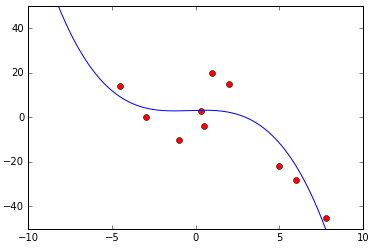
Plotting the original data against the least squares polynomial fit:

plt.axis([-10,10,-50,50])
plt.plot(xa,ya,'ro')
x=np.arange(-10,10,0.1)
y=np.array(-0.1020*x**3-0.1178*x**2+0.2065*x+3.063)
plt.plot(x,y)


Next Up
In the next article we will use polynomial interpolation to perform trend analysis.